Understanding Industrial Robot Motion Types

Introduction

Moving a robot from point A to point B seems like one of the most simple tasks you can program a robot to do. While this statement, in a sense, is true, the specific motion command used to get from point A to point B is extremely important and, if programmed incorrectly, can lead to some quite unfortunate and dangerous accidents.

This tutorial will cover the basics of robot motion commands, their workings, and their applications in industry. We will then learn about continuous and approximation of robot motions. 

By the end of this tutorial, you will understand which motion type to use and when to use it.

Industrial robots use three basic motion types, which most manufacturers share. These are "Point to Point (PTP or JOINT)," "Linear," and "CIRC or ARC" motions.

Linear Motion

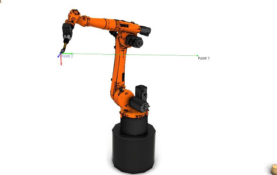
A “Linear” motion is the most understandable of all robot motions. As the name suggests, this type of motion is a simple straight line from "Point 1" to "Point 2". As shown in “Figure 1”, the robot will travel straight from its current position to its end position, maintaining that the robot TCP (Tool Center Point) will stay on the straight path (shown in green). 

This specific type of motion can be necessary for many applications. For example, when moving in a very tight or confined space where you cannot allow the robot too much freedom in its movement. A “Linear” motion is also necessary when offsetting another point by a set amount or traveling along a seam, weld, milling path, or drilling a hole.

The robot rotates all its joints to maintain its correct path. Still, there can be many disadvantages to this as well as advantages depending on the application.

One of the main disadvantages of a “Linear” motion is that it tends to be slower than a standard “PTP” or “Joint” movement. This is because some joints will need to move more than others to keep the robot on its straight path, depending on the specific orientation of the robot and its current joint positions. 

The motion will always be limited by the maximum speed of the slowest moving joint as each of the joint motors will have a top speed.

Let’s take the robot in "Figure 1" and set 3 m/s as the maximum joint speed for all axes. 

Suppose we program the robot to move from "Point 1" to "Point 2" with a TCP speed of 2 m/s. To maintain this speed on the robot TCP, the robot axes will need to move in unison and at varying speeds. In some cases, the speed of one of the axes may need to move beyond the axis speed limit. In this case, axis 4, for example, moves beyond 3m/s. This speed is beyond the axis limit, so to prevent errors, including overload, the robot will need to lower the TCP speed to allow this limitation on axis 4. In this specific situation, the TCP speed would need to be reduced by roughly 40% to 1.2 m/s to account for the axis limitations.

Point to Point (JOINT) Motion

A “Point to Point” motion will have the same result as a “Linear” motion, but the robot's path to achieving this will be different as the robot will not move along or maintain a straight path. 

“Point to Point” motions are accomplished using the fastest rather than the shortest path. 

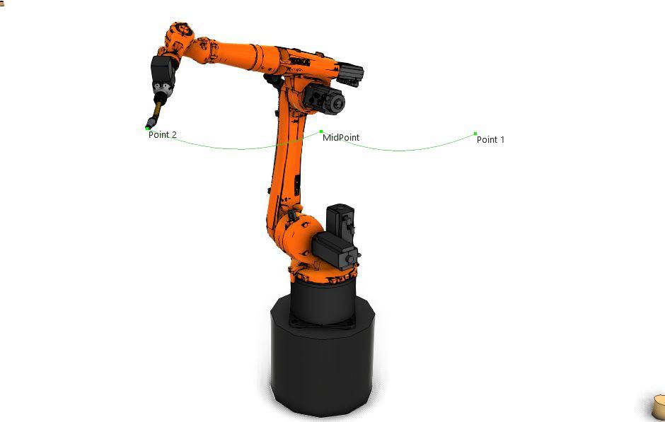
For example, as shown in "Figure 2," the same points are used as in "Figure 1," but the robot takes a different non-linear path, arcing toward "Point 2" instead of traveling straight. This path may be longer but results in a shorter movement time. 

Using “Point to Point” motions is advantageous as it allows the robot joints to move at their highest programmable velocity. It enables the user to optimize the robot's operation and reduce the cycle time. However, these movements are much more unpredictable than “Linear” motions.

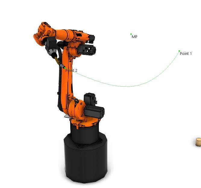
For example, "Figure 3" shows an example of the Point-to-Point move unpredictability; an additional point has now been added to the path, "MidPoint." This single point has now drastically changed the arcing path from "Figure 2". This shows that the robot's entire motion sequence must be checked when teaching point-to-point motions, not just the points themselves.

You cannot easily predict the robot's path to reach its destination points during a point-to-point move, so you must take extra care.

Unconstrained point-to-point motions fit very well in applications with abundant space, for example, palletizing applications, as you can give the robot the freedom to perform arcing motions to get to its required destination. 

These motions also work in applications where the space is restricted, but the movements must be limited. You can do this by using a fixed speed in the program's specific area and fixed unchanging point locations, as these two items can vary the robot's path if changed. 

Another option is to increase the number of points on the robot path to constrain it but still allow variation in the motion between them. Increasing the points constrains the robot to a somewhat steady path but allows the freedom to vary and move on a non-linear path between these point locations. Still, it can have the side effect of slowing the robot down as it will still need to come close to these new positions even if it is allowed to approximate.

CIRC or ARC Motion

A “CIRC” (circular or ARC) motion drives the robot's TCP from the start to the end of its move in a constant radius. “CIRC” motion is used for many standard applications, including milling, gluing, welding, etc.

This motion is executed by teaching the robot a minimum of 2 positions, an endpoint, and an auxiliary point. The robot will then move in a circular arc from the end of its previous move through the auxiliary position and to its end position in a circular arc. 

The accuracy of the circle achieved through this motion depends on the placement of these points. The best practice is teaching the “Aux” point close to the arc's center point. 

When using a “CIRC” motion, a complete circle is also not always needed. For example, the programmer can use this motion type to make full circles or finite arcs depending on the specific application.

Motion Approximation

When a robot moves through a set of standard points, it will stop at each point, reducing a system's cycle time. The constant deceleration and acceleration are hard on the robot's mechanics. A motion can be programmed using approximated motions to avoid this problem. 

Allowing the robot to approximate a point coordinate will accelerate the entire motion sequence. Instead of stopping on the exact point coordinate, the robot will leave the path before reaching a point and begin its motion toward the next point in the sequence. 

The level of approximation of a motion can be programmed. This approximation is programmed by specifying a distance the robot can leave its programmed path before and after the point or by selecting a percentage of the moving distance.

The sequence of images  "Figure 5", "Figure 6", Figure 7," and "Figure 8" explains the approximation of a robot motion.

"Figure 5" shows a robot motion starting at "Point 1" and moving through "MidPoint" to get to "Point 2". No approximation has been programmed for this movement so that the robot will stop at all points on its path exactly or as close as the robot's physical accuracy allows. 

In "Figure 6," the robot moves along the same path as in “Figure 5”. Instead of moving and stopping directly on the "MidPoint," the robot deviates 50mm before and after the “MidPoint”. This is because of a 50mm approximation programmed into its motion command. 

In "Figure 7" and "Figure 8," it is shown that as we increase the approximation distance, in this case to 150mm and 500mm, respectively, the motion becomes much more similar to the standard “PTP” move. The robot now moves as if the midpoint did not exist, forming a sizeable sweeping motion directly from "Point 1" to "Point 2" avoiding the "MidPoint" altogether. 

The approximation of a motion is vital in many applications as the cycle time constraints may require it, and it is good practice to use for smooth paths. Still, as you can see, if the distance is programmed to be too large, then the motion approximation becomes pointless. There is a limitation regarding the maximum approximation distance allowed on a motion. 

“Figure 9” shows a set of three points, “P1”, “MP,” and “P3”. “P1” and “P3” are equidistant from “MP” at a distance of 150mm. Therefore, if we programmed the robot to move from “P1” to “P3” on this standard path without any approximation, the total motion length would be 300mm.

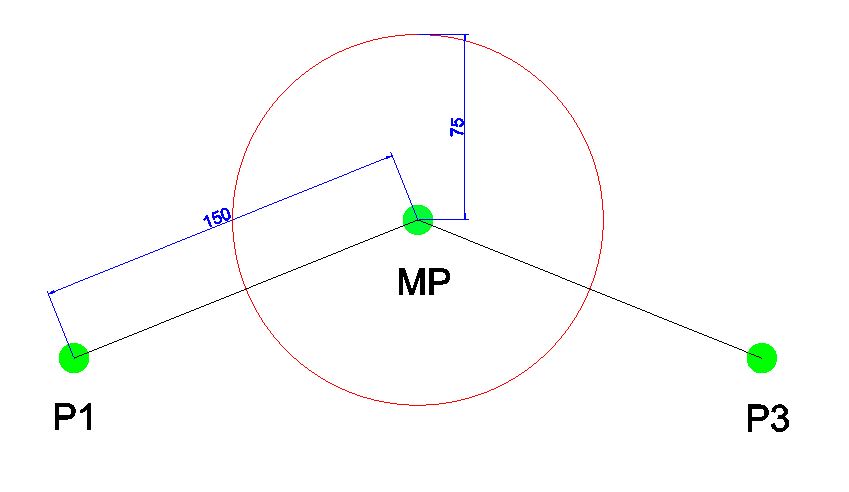
“Figure 10” shows the same path as “Figure 9,” but an approximation has been programmed at “MP.” This approximation is programmed using a distance of 75mm, shown by the circle surrounding “MP.” This means that the robot can begin to leave the standard path 75mm before the point but needs to be back on the standard path 75mm after the point. 

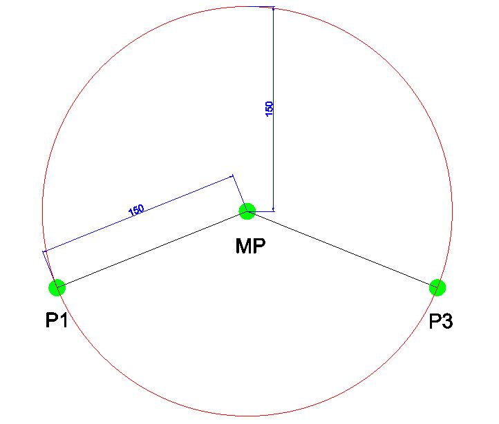
"Figure 11" again shows the same path, but an approximation has been programmed at "MP" using a distance of 150mm. Since "P1" and "P3" are both 150mm from "MP," this means that the robot can leave its standard path directly at "P1" and only return to this path directly on "P3". This sets our approximation limit at this point in this motion as if the value was programmed to be greater than 150mm; the robot would not be able to reach "P3," making the motion non-viable. 

This general limit on approximation is defined at a maximum of half the entire motion distance without approximation.

Conclusion

This tutorial has covered the basics of robot motion types. You learned that there are various tools that you can use to get the robot from A to B. Linear motions move the robot in a straight line from A to B. Point to Point motions move the robot in the fasted path from A to B, and CIRC motions move the robot TCP in an arc. The motion type used depends on the robot application and application environment. This tutorial has also covered the basics of motion approximation and how it can be used to reduce a robot's motion time. By now, you should better understand these motion types, how they work, and where you could use them.